So, given the ability to build a jump table for a range of inputs, it would be useful to transform a given input value onto one of the valid options for that table. If you have a quick look at the pseudo code reproduced from Wikipedia, you’ll see it has a validate x instruction, which if you ask me is an unapologetically brief way of describing a hashing, bounding, clamping or range-checking process. However, that’s what this post is about: confining an input to a range of output values. It’s actually unrelated to the generation or use of a jump table, but it doesn’t take much imagination to see how it might be useful.
The other thing which bears mentioning is that this can easily be accomplished by using conditionals, e.g.:
cmp %rax, %rdx
jge .Lgt_or_eq
The thing is, though, that I can’t see any point in going to the trouble of writing a routine in assembler if you’re not going to do so elegantly and efficiently. And the following technique is both efficient and elegant and the brainchild of someone far more intelligent than me.
It’s reasonably well understood that conditional branches will, for the most part, cause code to execute more slowly than non-branching code. This is due to branch prediction and instruction pipelines. A CPU’s branch predictor will attempt to guess which of the two code-paths following a conditional branch is more likely to occur and speculatively execute that path. If it guesses correctly, it’s ahead of the game, but if it guesses incorrectly, the evaluation is wasted and it will stall while it refills its pipeline with the right instructions it needs to execute.
This method of constraining a set of inputs onto a range of outputs does so without any conditional instructions at all, and should produce a consistent evaluation time while a routine with conditional code would probably demonstrate much slower outlier values.
Given a range of outputs between 0 and 4, where the value 4 could be thought of as being the ‘default’ case, given switch-block terminology, the following assembly program will produce the following outputs given these inputs:
| Input | Output | Bitmask |
|---|---|---|
| -1 | 4 | 0 |
| 0 | 0 | -1 |
| 1 | 1 | -1 |
| 2 | 2 | -1 |
| 3 | 3 | -1 |
| 4 | 4 | 0 |
| 5 | 4 | 0 |
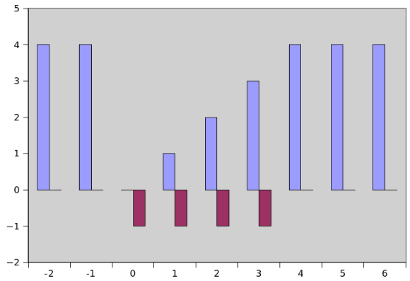
These values can also be represented graphically, for example as per the chart below. The chart is intended to convey how the output values (the y-axis and blue columns) vary with the intput value (on the x-axis). The maroon columns show the value of a bitmask generated using the technique.
It’s probably easier at this point to show the assembly for this technique before getting into a discussion of how it works. Here it is:
bounds.s
.section .rodata
output:
 .asciz "The result was %d\n"
upper:
 .quad 0x4           # p/t upper: binary 100
input:
 .quad 0x0
.section .text

.globl _start

_start:

 mov %rsp, %rbp

 leaq 0x10(%rbp), %rdi
 movq (%rdi), %rdi
 call atoi

 movq %rax, %rdx        # copy RAX into RDX
 subq upper, %rax       # subtract 'upper' from the input value
 sbb  %rax, %rax        # subtract RAX (with-borrow) from itself. RAX becomes either 0 or -1.
 and  %rax, %rdx        # use RAX as a mask to clear or preserve the bits in RDX
 not  %rax              # invert the bits in RAX. RAX is either -1 or 0.
 andq upper, %rax       # set RAX = 0 or value of 'upper'
 add  %rax, %rdx        #

 movq $output, %rdi     # Output the result
 movq %rdx, %rsi
 movq $1, %rax
 call printf

 movq $60, %rax
 movq $0, %rdi
 syscall
Makefile
bounds: bounds.o
 ld --dynamic-linker /lib/ld-linux-x86-64.so.2 -o bounds bounds.o -lc

bounds.o: bounds.s
 as -gstabs -o bounds.o bounds.s

clean:
 rm -f \*.o bounds
..
So how does this work? Well, the original algorithm designer understood how to use the carry flag to identify those values which fell within his target range and by using a masking technique cause the output to be bounded as desired.
By way of example, let’s walk through what happens for the values ‘1’ and ‘5’ as the argument to the program above. Let’s start just after the instruction
movq %rax, %rdxwhen both %rax and %rdx contain the input value. The instruction
subq upper, %rax has the effect of setting the carry flag if the input value is between zero and upper; otherwise, the carry flag is cleared. That’s all we’re interested in since the next operation effectively discards the result held in %rax. To continue our example, an input of 1 results in -3 and the carry flag being set while an input of 5 results in 1 and the carry flag being cleared.
The next instruction
sbb %rax, %rax subtracts %rax from itself, yielding zero, but crucially then subtracts 1 from that value if the carry flag is set. For an input of 1, %rax now contains -1 (or 11111111..._[etc]_...1111), while for an input of 5 it contains zero.
The rest of the algorithm uses the bitmask to generate a bounded output value. The next instruction
and %rax, %rdx clears or retains the value stored in %rdx (since the %rax operand can contain only zero or -1). For an input of 1, %rdx continues to contain 1, while for an input of 5, it is cleared and equal to zero.
The instruction
not %rax inverts the bits contained in %rax. For input 1, %rax contains 0, for an input of 5 it contains -1.
The penultimate instruction
`andq upper, %rax` sets up %rax to contain either the upper-bound or zero; for an input of 1 it contains zero since %rax is zero, while for an input of 5, %rax now contains 4 (the upper bound) since %rax is -1.
The final instruction
add %rax, %rdx yields the result by adding the value in %rax (zero or the value in upper) to %rdx (the original input, or zero). For an input of 1, this results in 1 (as rax:0 + rdx:1), while for an input of 5, this results in 4 (rax:4 + rdx:0).
I find this algorithm fairly confusing, especially if I try to explain it to someone without the benefit of some paper. The good news is that it also works for negative input values: these are treated as out-of-bounds and result in the upper-bound being returned.
I hope you were as fascinated by the apparent slight of hand as I am, and that I managed to explain it well enough! Many thanks to Scali of the asmcommunity.net forum for reminding me of the algorithm.
2011-10-21: I think I’ve found the discussion where I originally came across the technique.